PyTorch训练神经网络

可以使用torch.nn包来构建神经网络。

nn包则依赖于autograd包来定义模型并对它们求导。一个nn.Module包含各个层和一个forward(input)方法，该方法返回output。

如图这个神经网络可以对数字进行分类：

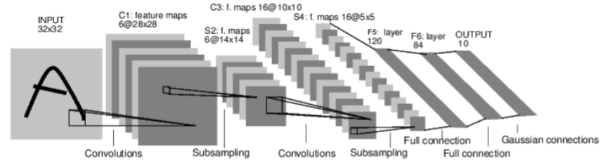
这是一个简单的前馈神经网络 (feed-forward network）。它接受一个输入，然后将它送入下一层，一层接一层的传递，最后给出输出。

一个神经网络的典型训练过程如下：

• 定义包含一些可学习参数(或者叫权重）的神经网络
• 在输入数据集上迭代
• 通过网络处理输入
• 计算 loss (输出和正确答案的距离）
• 将梯度反向传播给网络的参数
• 更新网络的权重，一般使用一个简单的规则：$$weight = weight - learning_rate * gradient。$$

定义神经网络

import torch
import torch.nn as nn
import torch.nn.functional as F

导包后定义神经网络：

class Net(nn.Module):
    def __init__(self):
        super(Net, self).__init__()
        # 输入图像channel：1；输出channel：6；5x5卷积核
        self.conv1 = nn.Conv2d(1, 6, 5)
        self.conv2 = nn.Conv2d(6, 16, 5)
        # an affine operation: y = Wx + b
        self.fc1 = nn.Linear(16 * 5 * 5, 120)
        self.fc2 = nn.Linear(120, 84)
        self.fc3 = nn.Linear(84, 10)

    def forward(self, x):
        # 2x2 Max pooling
        x = F.max_pool2d(F.relu(self.conv1(x)), (2, 2))
        # 如果是方阵,则可以只使用一个数字进行定义
        x = F.max_pool2d(F.relu(self.conv2(x)), 2)
        x = x.view(-1, self.num_flat_features(x))
        x = F.relu(self.fc1(x))
        x = F.relu(self.fc2(x))
        x = self.fc3(x)
        return x
    def num_flat_features(self, x):
        size = x.size()[1:]  # 除去批处理维度的其他所有维度
        num_features = 1
        for s in size:
            num_features *= s
        return num_features

测试：

net = Net()
print(net)

输出：

Net(
  (conv1): Conv2d(1, 6, kernel_size=(5, 5), stride=(1, 1))
  (conv2): Conv2d(6, 16, kernel_size=(5, 5), stride=(1, 1))
  (fc1): Linear(in_features=400, out_features=120, bias=True)
  (fc2): Linear(in_features=120, out_features=84, bias=True)
  (fc3): Linear(in_features=84, out_features=10, bias=True)
)

个模型的可学习参数可以通过net.parameters()返回:

params = list(net.parameters())
print(len(params))
print(params[0].size())  # conv1's .weight

输出：

10
torch.Size([6, 1, 5, 5])

将一个随机的 32x32作为输入。这个网络 (LeNet）的期待输入是 32x32 的张量。如果使用 MNIST 数据集来训练这个网络，要把图片大小重新调整到 32x32。

input = torch.randn(1, 1, 32, 32)
out = net(input)
print(out)

输出为：

tensor([[ 0.0399, -0.0856,  0.0668,  0.0915,  0.0453, -0.0680, -0.1024,  0.0493,
         -0.1043, -0.1267]], grad_fn=<AddmmBackward>)

清零所有参数的梯度缓存，然后进行随机梯度的反向传播：

net.zero_grad()
out.backward(torch.randn(1, 10))

torch.nn只支持小批量处理 (mini-batches）。整个 torch.nn 包只支持小批量样本的输入，不支持单个样本的输入。比如，nn.Conv2d 接受一个4维的张量，即nSamples x nChannels x Height x Width 如果是一个单独的样本，只需要使用input.unsqueeze(0)来添加一个“假的”批大小维度。

损失函数

一个损失函数接受一对(output, target)作为输入，计算一个值来估计网络的输出和目标值相差多少。

nn包中有很多不同的损失函数。nn.MSELoss是比较简单的一种，它计算输出和目标的均方误差。例如：

output = net(input)
target = torch.randn(10)  # 本例子中使用模拟数据
target = target.view(1, -1)  # 使目标值与数据值尺寸一致
criterion = nn.MSELoss()

loss = criterion(output, target)
print(loss)

输出：

tensor(1.0263, grad_fn=<MseLossBackward>)

现在，如果使用loss的.grad_fn属性跟踪反向传播过程，会看到计算图如下：

input -> conv2d -> relu -> maxpool2d -> conv2d -> relu -> maxpool2d
      -> view -> linear -> relu -> linear -> relu -> linear
      -> MSELoss
      -> loss

反向传播

我们只需要调用loss.backward()来反向传播误差。我们需要清零现有的梯度，否则梯度将会与已有的梯度累加。

现在，我们将调用loss.backward()，并查看 conv1层的偏置在反向传播前后的梯度。

net.zero_grad()     # 清零所有参数(parameter）的梯度缓存

print('conv1.bias.grad before backward')
print(net.conv1.bias.grad)

loss.backward()

print('conv1.bias.grad after backward')
print(net.conv1.bias.grad)

输出：

conv1.bias.grad before backward
tensor([0., 0., 0., 0., 0., 0.])
conv1.bias.grad after backward
tensor([ 0.0084,  0.0019, -0.0179, -0.0212,  0.0067, -0.0096])

更新权重

最简单的更新规则是随机梯度下降法 (SGD）:

weight = weight - learning_rate * gradient

torch.optim中实现了所有的这些方法。使用它很简单：

import torch.optim as optim

# 创建优化器(optimizer）
optimizer = optim.SGD(net.parameters(), lr=0.01)

# 在训练的迭代中：
optimizer.zero_grad()   # 清零梯度缓存
output = net(input)
loss = criterion(output, target)
loss.backward()
optimizer.step()    # 更新参数

训练一个图片分类器

以训练一个图片分类器为实例，按照上述步骤进行：

加载数据集

import torch
import torchvision
import torchvision.transforms as transforms

transform = transforms.Compose(
    [transforms.ToTensor(),
     transforms.Normalize((0.5, 0.5, 0.5), (0.5, 0.5, 0.5))])

trainset = torchvision.datasets.CIFAR10(root='./data', train=True, download=True, transform=transform)
trainloader = torch.utils.data.DataLoader(trainset, batch_size=4, shuffle=True, num_workers=2)

testset = torchvision.datasets.CIFAR10(root='./data', train=False, download=True, transform=transform)
testloader = torch.utils.data.DataLoader(testset, batch_size=4, shuffle=False, num_workers=2)

classes = ('plane', 'car', 'bird', 'cat',
           'deer', 'dog', 'frog', 'horse', 'ship', 'truck')

可视化数据

import matplotlib.pyplot as plt
import numpy as np

# 输出图像的函数
def imshow(img):
    img = img / 2 + 0.5     # unnormalize
    npimg = img.numpy()
    plt.imshow(np.transpose(npimg, (1, 2, 0)))
    plt.show()


# 随机获取训练图片
dataiter = iter(trainloader)
images, labels = dataiter.next()

# 显示图片
imshow(torchvision.utils.make_grid(images))
# 打印图片标签
print(' '.join('%5s' % classes[labels[j]] for j in range(4)))

定义一个卷积神经网络

将最初定义的神经网络拿过来，并将其修改成输入为3通道图像(替代原来定义的单通道图像）。

import torch.nn as nn
import torch.nn.functional as F


class Net(nn.Module):
    def __init__(self):
        super(Net, self).__init__()
        self.conv1 = nn.Conv2d(3, 6, 5)
        self.pool = nn.MaxPool2d(2, 2)
        self.conv2 = nn.Conv2d(6, 16, 5)
        self.fc1 = nn.Linear(16 * 5 * 5, 120)
        self.fc2 = nn.Linear(120, 84)
        self.fc3 = nn.Linear(84, 10)

    def forward(self, x):
        x = self.pool(F.relu(self.conv1(x)))
        x = self.pool(F.relu(self.conv2(x)))
        x = x.view(-1, 16 * 5 * 5)
        x = F.relu(self.fc1(x))
        x = F.relu(self.fc2(x))
        x = self.fc3(x)
        return x


net = Net()

定义损失函数和优化器

使用多分类的交叉熵损失函数和随机梯度下降优化器：

import torch.optim as optim

criterion = nn.CrossEntropyLoss()
optimizer = optim.SGD(net.parameters(), lr=0.001, momentum=0.9)

训练网络

遍历数据迭代器，并将输入“喂”给网络和优化函数。

for epoch in range(2):  # loop over the dataset multiple times

    running_loss = 0.0
    for i, data in enumerate(trainloader, 0):
        # get the inputs
        inputs, labels = data

        # zero the parameter gradients
        optimizer.zero_grad()

        # forward + backward + optimize
        outputs = net(inputs)
        loss = criterion(outputs, labels)
        loss.backward()
        optimizer.step()

        # print statistics
        running_loss += loss.item()
        if i % 2000 == 1999:    # print every 2000 mini-batches
            print('[%d, %5d] loss: %.3f' % (epoch + 1, i + 1, running_loss / 2000))
            running_loss = 0.0

print('Finished Training')

保存训练好的模型：

PATH = './cifar_net.pth'
torch.save(net.state_dict(), PATH)

使用测试数据测试网络

将通过预测神经网络输出的标签来检查这个问题，并和正确样本进行对比。如果预测是正确的，将样本添加到正确预测的列表中。

dataiter = iter(testloader)
images, labels = dataiter.next()

# 输出图片
imshow(torchvision.utils.make_grid(images))
print('GroundTruth: ', ' '.join('%5s' % classes[labels[j]] for j in range(4)))

加载保存的模型：

net = Net()
net.load_state_dict(torch.load(PATH))

神经网络认为上面的例子是:

outputs = net(images)

输出是10个类别的量值。一个类的值越高，网络就越认为这个图像属于这个特定的类。让我们得到最高量值的下标/索引；

_, predicted = torch.max(outputs, 1)

print('Predicted: ', ' '.join('%5s' % classes[predicted[j]] for j in range(4)))

结果对比：

GroundTruth:    cat  ship  ship plane
Predicted:    dog  ship  ship plane

correct = 0
total = 0
with torch.no_grad():
    for data in testloader:
        images, labels = data
        outputs = net(images)
        _, predicted = torch.max(outputs.data, 1)
        total += labels.size(0)
        correct += (predicted == labels).sum().item()

print('Accuracy of the network on the 10000 test images: %d %%' % (
    100 * correct / total))

观测整个数据集上的表现：

correct = 0
total = 0
with torch.no_grad():
    for data in testloader:
        images, labels = data
        outputs = net(images)
        _, predicted = torch.max(outputs.data, 1)
        total += labels.size(0)
        correct += (predicted == labels).sum().item()

print('Accuracy of the network on the 10000 test images: %d %%' % (
    100 * correct / total))

输出结果：

Accuracy of the network on the 10000 test images: 55 %

这比随机选取(即从10个类中随机选择一个类，正确率是10%）要好很多。看来网络确实学到了一些东西。接着看看具体是哪些表现的差的类呢？

class_correct = list(0. for i in range(10))
class_total = list(0. for i in range(10))
with torch.no_grad():
    for data in testloader:
        images, labels = data
        outputs = net(images)
        _, predicted = torch.max(outputs, 1)
        c = (predicted == labels).squeeze()
        for i in range(4):
            label = labels[i]
            class_correct[label] += c[i].item()
            class_total[label] += 1


for i in range(10):
    print('Accuracy of %5s : %2d %%' % (
        classes[i], 100 * class_correct[i] / class_total[i]))

GPU跑pytorch

用GPU跑pytorch程序就3点：

1. 申明用GPU
2. 把你的model放到GPU上
3. 把数据和标签放到GPU上

申明

device=torch.device('cuda' if torch.cuda.is_available() else 'cpu')
print(device)

将模型放到GPU上

在创建完网络 或者引用网络之后，我们需要实体化我们的网络。直接在后面加一句话就可以

net= Net ()
net.to(device)

把数据放到GPU上

inputs, labels = data
            inputs, labels = inputs.to(device), labels.to(device)

最后可以用nvidia-smi查看是否利用gpu训练。