import numpy as np
import pandas as pd
生成对象
- Series:维度——1;带标签的一维同构数组
- DataFrame:维度——2;带标签的,大小可变的,二维异构表格
s = pd.Series([1, 3, 5, np.nan, 6, 8])
s
0    1.0
1    3.0
2    5.0
3    NaN
4    6.0
5    8.0
dtype: float64
含日期时间:
datas = pd.date_range('20130101', periods=6)
datas
DatetimeIndex(['2013-01-01', '2013-01-02', '2013-01-03', '2013-01-04',
               '2013-01-05', '2013-01-06'],
              dtype='datetime64[ns]', freq='D')
含日期时间索引与标签的 NumPy 数组生成DataFrame
df = pd.DataFrame(np.random.randn(6,4),index=datas, columns=list('ABCD'))
df
|
A |
B |
C |
D |
| 2013-01-01 |
0.477423 |
0.183968 |
-0.139705 |
-0.727223 |
| 2013-01-02 |
-0.168761 |
-0.922938 |
0.396889 |
-2.779128 |
| 2013-01-03 |
-0.618984 |
0.576812 |
1.900378 |
-0.624996 |
| 2013-01-04 |
-1.395511 |
0.525819 |
0.112159 |
-0.160826 |
| 2013-01-05 |
0.280020 |
-2.186553 |
-0.644597 |
1.163917 |
| 2013-01-06 |
1.945874 |
0.014268 |
-1.506800 |
0.405446 |
用字典对象生成DataFrame
df2 = pd.DataFrame({'A': 1.,
                    'B': pd.Timestamp('20130102'),
                    'C': pd.Series(1,index=list(range(4))),
                    'D': np.array([3]*4, dtype='int32'),
                    'E': pd.Categorical(["test", "train", "test", "train"]),
                    'F': 'foo'})
df2
|
A |
B |
C |
D |
E |
F |
| 0 |
1.0 |
2013-01-02 |
1 |
3 |
test |
foo |
| 1 |
1.0 |
2013-01-02 |
1 |
3 |
train |
foo |
| 2 |
1.0 |
2013-01-02 |
1 |
3 |
test |
foo |
| 3 |
1.0 |
2013-01-02 |
1 |
3 |
train |
foo |
df2.dtypes
A           float64
B    datetime64[ns]
C             int64
D             int32
E          category
F            object
dtype: object
df.head()
|
A |
B |
C |
D |
| 2013-01-01 |
0.477423 |
0.183968 |
-0.139705 |
-0.727223 |
| 2013-01-02 |
-0.168761 |
-0.922938 |
0.396889 |
-2.779128 |
| 2013-01-03 |
-0.618984 |
0.576812 |
1.900378 |
-0.624996 |
| 2013-01-04 |
-1.395511 |
0.525819 |
0.112159 |
-0.160826 |
| 2013-01-05 |
0.280020 |
-2.186553 |
-0.644597 |
1.163917 |
df.info
<bound method DataFrame.info of                    A         B         C         D
2013-01-01  0.477423  0.183968 -0.139705 -0.727223
2013-01-02 -0.168761 -0.922938  0.396889 -2.779128
2013-01-03 -0.618984  0.576812  1.900378 -0.624996
2013-01-04 -1.395511  0.525819  0.112159 -0.160826
2013-01-05  0.280020 -2.186553 -0.644597  1.163917
2013-01-06  1.945874  0.014268 -1.506800  0.405446>
df.tail(3)
|
A |
B |
C |
D |
| 2013-01-04 |
-1.395511 |
0.525819 |
0.112159 |
-0.160826 |
| 2013-01-05 |
0.280020 |
-2.186553 |
-0.644597 |
1.163917 |
| 2013-01-06 |
1.945874 |
0.014268 |
-1.506800 |
0.405446 |
df.index
DatetimeIndex(['2013-01-01', '2013-01-02', '2013-01-03', '2013-01-04',
               '2013-01-05', '2013-01-06'],
              dtype='datetime64[ns]', freq='D')
df.columns
Index(['A', 'B', 'C', 'D'], dtype='object')
DataFrame.to_numpy() 输出底层数据的 NumPy 对象。注意,DataFrame的列由多种数据类型组成时,该操作耗费系统资源较大,这也是Pandas和NumPy的本质区别:NumPy数组只有一种数据类型,DataFrame每列的数据类型各不相同。调用 DataFrame.to_numpy()时,Pandas 查找支持DataFrame里所有数据类型的NumPy数据类型。还有一种数据类型是object,可以把DataFrame列里的值强制转换为Python对象。
df.to_numpy()
array([[ 0.47742267,  0.18396775, -0.13970455, -0.72722311],
       [-0.168761  , -0.92293827,  0.3968894 , -2.77912839],
       [-0.6189843 ,  0.57681245,  1.90037812, -0.62499646],
       [-1.3955112 ,  0.52581862,  0.11215897, -0.16082579],
       [ 0.2800197 , -2.18655291, -0.64459677,  1.16391673],
       [ 1.94587401,  0.01426759, -1.50679977,  0.40544621]])
df2.to_numpy()
array([[1.0, Timestamp('2013-01-02 00:00:00'), 1, 3, 'test', 'foo'],
       [1.0, Timestamp('2013-01-02 00:00:00'), 1, 3, 'train', 'foo'],
       [1.0, Timestamp('2013-01-02 00:00:00'), 1, 3, 'test', 'foo'],
       [1.0, Timestamp('2013-01-02 00:00:00'), 1, 3, 'train', 'foo']],
      dtype=object)
df.describe()
|
A |
B |
C |
D |
| count |
6.000000 |
6.000000 |
6.000000 |
6.000000 |
| mean |
0.086677 |
-0.301437 |
0.019721 |
-0.453802 |
| std |
1.131969 |
1.070597 |
1.138830 |
1.338086 |
| min |
-1.395511 |
-2.186553 |
-1.506800 |
-2.779128 |
| 25% |
-0.506428 |
-0.688637 |
-0.518374 |
-0.701666 |
| 50% |
0.055629 |
0.099118 |
-0.013773 |
-0.392911 |
| 75% |
0.428072 |
0.440356 |
0.325707 |
0.263878 |
| max |
1.945874 |
0.576812 |
1.900378 |
1.163917 |
df.T
|
2013-01-01 |
2013-01-02 |
2013-01-03 |
2013-01-04 |
2013-01-05 |
2013-01-06 |
| A |
0.477423 |
-0.168761 |
-0.618984 |
-1.395511 |
0.280020 |
1.945874 |
| B |
0.183968 |
-0.922938 |
0.576812 |
0.525819 |
-2.186553 |
0.014268 |
| C |
-0.139705 |
0.396889 |
1.900378 |
0.112159 |
-0.644597 |
-1.506800 |
| D |
-0.727223 |
-2.779128 |
-0.624996 |
-0.160826 |
1.163917 |
0.405446 |
按轴排序
df2.sort_index(axis=1,ascending=False)
|
F |
E |
D |
C |
B |
A |
| 0 |
foo |
test |
3 |
1 |
2013-01-02 |
1.0 |
| 1 |
foo |
train |
3 |
1 |
2013-01-02 |
1.0 |
| 2 |
foo |
test |
3 |
1 |
2013-01-02 |
1.0 |
| 3 |
foo |
train |
3 |
1 |
2013-01-02 |
1.0 |
按值排序
df.sort_values(by='B')
|
A |
B |
C |
D |
| 2013-01-05 |
0.280020 |
-2.186553 |
-0.644597 |
1.163917 |
| 2013-01-02 |
-0.168761 |
-0.922938 |
0.396889 |
-2.779128 |
| 2013-01-06 |
1.945874 |
0.014268 |
-1.506800 |
0.405446 |
| 2013-01-01 |
0.477423 |
0.183968 |
-0.139705 |
-0.727223 |
| 2013-01-04 |
-1.395511 |
0.525819 |
0.112159 |
-0.160826 |
| 2013-01-03 |
-0.618984 |
0.576812 |
1.900378 |
-0.624996 |
选择
df['A']
2013-01-01    0.477423
2013-01-02   -0.168761
2013-01-03   -0.618984
2013-01-04   -1.395511
2013-01-05    0.280020
2013-01-06    1.945874
Freq: D, Name: A, dtype: float64
df[0:3]
|
A |
B |
C |
D |
| 2013-01-01 |
0.477423 |
0.183968 |
-0.139705 |
-0.727223 |
| 2013-01-02 |
-0.168761 |
-0.922938 |
0.396889 |
-2.779128 |
| 2013-01-03 |
-0.618984 |
0.576812 |
1.900378 |
-0.624996 |
df['2013-01-02':'20130104'] ## 时间的这两种书写方式一样
|
A |
B |
C |
D |
| 2013-01-02 |
-0.168761 |
-0.922938 |
0.396889 |
-2.779128 |
| 2013-01-03 |
-0.618984 |
0.576812 |
1.900378 |
-0.624996 |
| 2013-01-04 |
-1.395511 |
0.525819 |
0.112159 |
-0.160826 |
按标签选择
df.loc[datas[0]]
A    0.477423
B    0.183968
C   -0.139705
D   -0.727223
Name: 2013-01-01 00:00:00, dtype: float64
df.loc[:,['A','B']]
# df[['A','B']]       ## 等同
|
A |
B |
| 2013-01-01 |
0.477423 |
0.183968 |
| 2013-01-02 |
-0.168761 |
-0.922938 |
| 2013-01-03 |
-0.618984 |
0.576812 |
| 2013-01-04 |
-1.395511 |
0.525819 |
| 2013-01-05 |
0.280020 |
-2.186553 |
| 2013-01-06 |
1.945874 |
0.014268 |
df.loc[datas[1]:datas[3], ['A', 'B']]
|
A |
B |
| 2013-01-02 |
-0.168761 |
-0.922938 |
| 2013-01-03 |
-0.618984 |
0.576812 |
| 2013-01-04 |
-1.395511 |
0.525819 |
df.loc[datas[0], 'A'] # 等同于df.at[datas[0], 'A']
0.4774226701301457
按位置选择(重要)
df.iloc[3]
A   -1.395511
B    0.525819
C    0.112159
D   -0.160826
Name: 2013-01-04 00:00:00, dtype: float64
df.iloc[[1,2,4],[0,2]]
|
A |
C |
| 2013-01-02 |
-0.168761 |
0.396889 |
| 2013-01-03 |
-0.618984 |
1.900378 |
| 2013-01-05 |
0.280020 |
-0.644597 |
df.iloc[:, 1:3]
|
B |
C |
| 2013-01-01 |
0.183968 |
-0.139705 |
| 2013-01-02 |
-0.922938 |
0.396889 |
| 2013-01-03 |
0.576812 |
1.900378 |
| 2013-01-04 |
0.525819 |
0.112159 |
| 2013-01-05 |
-2.186553 |
-0.644597 |
| 2013-01-06 |
0.014268 |
-1.506800 |
布尔索引(重要)
# df.A
df[df.A > 0]
|
A |
B |
C |
D |
| 2013-01-01 |
0.477423 |
0.183968 |
-0.139705 |
-0.727223 |
| 2013-01-05 |
0.280020 |
-2.186553 |
-0.644597 |
1.163917 |
| 2013-01-06 |
1.945874 |
0.014268 |
-1.506800 |
0.405446 |
df[df > 0]
|
A |
B |
C |
D |
| 2013-01-01 |
0.477423 |
0.183968 |
NaN |
NaN |
| 2013-01-02 |
NaN |
NaN |
0.396889 |
NaN |
| 2013-01-03 |
NaN |
0.576812 |
1.900378 |
NaN |
| 2013-01-04 |
NaN |
0.525819 |
0.112159 |
NaN |
| 2013-01-05 |
0.280020 |
NaN |
NaN |
1.163917 |
| 2013-01-06 |
1.945874 |
0.014268 |
NaN |
0.405446 |
isin()筛选(重要)
df2 = df.copy()
df2['E'] = ['one', 'one', 'two', 'three', 'four', 'three']
df2[df2['E'].isin(['two', 'four'])]
|
A |
B |
C |
D |
E |
| 2013-01-03 |
-0.618984 |
0.576812 |
1.900378 |
-0.624996 |
two |
| 2013-01-05 |
0.280020 |
-2.186553 |
-0.644597 |
1.163917 |
four |
缺失值
df1 = df.reindex(index=datas[0:4], columns=list(df.columns))
df1.iloc[[1,3],[0,2]] = np.nan
df1
|
A |
B |
C |
D |
| 2013-01-01 |
0.477423 |
0.183968 |
-0.139705 |
-0.727223 |
| 2013-01-02 |
NaN |
-0.922938 |
NaN |
-2.779128 |
| 2013-01-03 |
-0.618984 |
0.576812 |
1.900378 |
-0.624996 |
| 2013-01-04 |
NaN |
0.525819 |
NaN |
-0.160826 |
删除所有含缺失值的行:
df1.dropna(how='any')
|
A |
B |
C |
D |
| 2013-01-01 |
0.477423 |
0.183968 |
-0.139705 |
-0.727223 |
| 2013-01-03 |
-0.618984 |
0.576812 |
1.900378 |
-0.624996 |
填充缺失值
df1.fillna(value=5)
|
A |
B |
C |
D |
| 2013-01-01 |
0.477423 |
0.183968 |
-0.139705 |
-0.727223 |
| 2013-01-02 |
5.000000 |
-0.922938 |
5.000000 |
-2.779128 |
| 2013-01-03 |
-0.618984 |
0.576812 |
1.900378 |
-0.624996 |
| 2013-01-04 |
5.000000 |
0.525819 |
5.000000 |
-0.160826 |
提取nan值的布尔掩码
pd.isna(df1)
|
A |
B |
C |
D |
| 2013-01-01 |
False |
False |
False |
False |
| 2013-01-02 |
True |
False |
True |
False |
| 2013-01-03 |
False |
False |
False |
False |
| 2013-01-04 |
True |
False |
True |
False |
运算
统计
求每列的均值
df.mean()
A    0.086677
B   -0.301437
C    0.019721
D   -0.453802
dtype: float64
求每行的均值
df.mean(1)
2013-01-01   -0.051384
2013-01-02   -0.868485
2013-01-03    0.308302
2013-01-04   -0.229590
2013-01-05   -0.346803
2013-01-06    0.214697
Freq: D, dtype: float64
s = pd.Series([1, 3, 5, np.nan, 6, 8], index=datas)
s.shift(3)
2013-01-01    NaN
2013-01-02    NaN
2013-01-03    NaN
2013-01-04    1.0
2013-01-05    3.0
2013-01-06    5.0
Freq: D, dtype: float64
df.sub(s, axis='index') # 减法运算
|
A |
B |
C |
D |
| 2013-01-01 |
-0.522577 |
-0.816032 |
-1.139705 |
-1.727223 |
| 2013-01-02 |
-3.168761 |
-3.922938 |
-2.603111 |
-5.779128 |
| 2013-01-03 |
-5.618984 |
-4.423188 |
-3.099622 |
-5.624996 |
| 2013-01-04 |
NaN |
NaN |
NaN |
NaN |
| 2013-01-05 |
-5.719980 |
-8.186553 |
-6.644597 |
-4.836083 |
| 2013-01-06 |
-6.054126 |
-7.985732 |
-9.506800 |
-7.594554 |
df
|
A |
B |
C |
D |
| 2013-01-01 |
0.477423 |
0.183968 |
-0.139705 |
-0.727223 |
| 2013-01-02 |
-0.168761 |
-0.922938 |
0.396889 |
-2.779128 |
| 2013-01-03 |
-0.618984 |
0.576812 |
1.900378 |
-0.624996 |
| 2013-01-04 |
-1.395511 |
0.525819 |
0.112159 |
-0.160826 |
| 2013-01-05 |
0.280020 |
-2.186553 |
-0.644597 |
1.163917 |
| 2013-01-06 |
1.945874 |
0.014268 |
-1.506800 |
0.405446 |
df.apply(np.cumsum) # 累加操作
|
A |
B |
C |
D |
| 2013-01-01 |
0.477423 |
0.183968 |
-0.139705 |
-0.727223 |
| 2013-01-02 |
0.308662 |
-0.738971 |
0.257185 |
-3.506352 |
| 2013-01-03 |
-0.310323 |
-0.162158 |
2.157563 |
-4.131348 |
| 2013-01-04 |
-1.705834 |
0.363661 |
2.269722 |
-4.292174 |
| 2013-01-05 |
-1.425814 |
-1.822892 |
1.625125 |
-3.128257 |
| 2013-01-06 |
0.520060 |
-1.808625 |
0.118325 |
-2.722811 |
df.apply(lambda x: x.max() - x.min())
A    3.341385
B    2.763365
C    3.407178
D    3.943045
dtype: float64
直方图
s = pd.Series(np.random.randint(0, 7, size=10))
s
0    4
1    3
2    4
3    1
4    3
5    1
6    6
7    2
8    6
9    0
dtype: int32
s.value_counts()
4    2
3    2
1    2
6    2
2    1
0    1
dtype: int64
删除与合并(重要)
df.loc[:,'E']=1.
# df.drop(labels=['E'],axis=0)
df
|
A |
B |
C |
D |
E |
| 2013-01-01 00:00:00 |
0.477423 |
0.183968 |
-0.139705 |
-0.727223 |
1.0 |
| 2013-01-02 00:00:00 |
-0.168761 |
-0.922938 |
0.396889 |
-2.779128 |
1.0 |
| 2013-01-03 00:00:00 |
-0.618984 |
0.576812 |
1.900378 |
-0.624996 |
1.0 |
| 2013-01-04 00:00:00 |
-1.395511 |
0.525819 |
0.112159 |
-0.160826 |
1.0 |
| 2013-01-05 00:00:00 |
0.280020 |
-2.186553 |
-0.644597 |
1.163917 |
1.0 |
| 2013-01-06 00:00:00 |
1.945874 |
0.014268 |
-1.506800 |
0.405446 |
1.0 |
pieces = [df[:3], df[3:]]
pieces
[                            A         B         C         D    E
 2013-01-01 00:00:00  0.477423  0.183968 -0.139705 -0.727223  1.0
 2013-01-02 00:00:00 -0.168761 -0.922938  0.396889 -2.779128  1.0
 2013-01-03 00:00:00 -0.618984  0.576812  1.900378 -0.624996  1.0,
                             A         B         C         D    E
 2013-01-04 00:00:00 -1.395511  0.525819  0.112159 -0.160826  1.0
 2013-01-05 00:00:00  0.280020 -2.186553 -0.644597  1.163917  1.0
 2013-01-06 00:00:00  1.945874  0.014268 -1.506800  0.405446  1.0]
pd.concat(pieces)
连接
left = pd.DataFrame({'key': ['foo', 'foo'], 'lval': [1, 2]})
right = pd.DataFrame({'key': ['foo', 'foo'], 'rval': [4, 5]})
pd.merge(left, right, on='key')
|
key |
lval |
rval |
| 0 |
foo |
1 |
4 |
| 1 |
foo |
1 |
5 |
| 2 |
foo |
2 |
4 |
| 3 |
foo |
2 |
5 |
left = pd.DataFrame({'key': ['foo', 'bar'], 'lval': [1, 2]})
right = pd.DataFrame({'key': ['foo', 'bar'], 'rval': [4, 5]})
pd.merge(left, right, on='key')
|
key |
lval |
rval |
| 0 |
foo |
1 |
4 |
| 1 |
bar |
2 |
5 |
添加(Append)
df = pd.DataFrame(np.random.randn(8, 4), columns=['A', 'B', 'C', 'D'])
s = df.iloc[3]
df.append(s, ignore_index=True)
|
A |
B |
C |
D |
| 0 |
-1.282560 |
1.578933 |
-1.835089 |
-0.570793 |
| 1 |
0.129816 |
0.697800 |
0.418487 |
-0.253009 |
| 2 |
-1.009696 |
-0.800243 |
0.324064 |
0.574360 |
| 3 |
-0.162016 |
0.497039 |
0.298132 |
-1.076649 |
| 4 |
0.630602 |
-1.781916 |
0.668464 |
0.663769 |
| 5 |
0.737596 |
-1.690360 |
-0.545418 |
-0.846643 |
| 6 |
1.418491 |
-1.698654 |
0.474682 |
-0.825363 |
| 7 |
-1.020948 |
1.351000 |
1.288640 |
-0.098584 |
| 8 |
-0.162016 |
0.497039 |
0.298132 |
-1.076649 |
分组(Grouping)
“group by” 指的是涵盖下列一项或多项步骤的处理流程:
- 分割:按条件把数据分割成多组;
- 应用:为每组单独应用函数;
- 组合:将处理结果组合成一个数据结构。
df = pd.DataFrame({'A': ['foo', 'bar', 'foo', 'bar',
                          'foo', 'bar', 'foo', 'foo'],
                   'B': ['one', 'one', 'two', 'three',
                          'two', 'two', 'one', 'three'],
                   'C': np.random.randn(8),
                   'D': np.random.randn(8)})
df
|
A |
B |
C |
D |
| 0 |
foo |
one |
0.452364 |
0.296516 |
| 1 |
bar |
one |
-0.469170 |
-0.143944 |
| 2 |
foo |
two |
1.295369 |
-0.269286 |
| 3 |
bar |
three |
-0.198760 |
-0.871319 |
| 4 |
foo |
two |
0.726845 |
-0.584794 |
| 5 |
bar |
two |
-0.384160 |
0.197542 |
| 6 |
foo |
one |
-0.844166 |
2.579093 |
| 7 |
foo |
three |
-0.665659 |
-0.728335 |
df.groupby(['A', 'B']).sum()
|
|
C |
D |
| A |
B |
|
|
| bar |
one |
-0.469170 |
-0.143944 |
| three |
-0.198760 |
-0.871319 |
| two |
-0.384160 |
0.197542 |
| foo |
one |
-0.391803 |
2.875609 |
| three |
-0.665659 |
-0.728335 |
| two |
2.022214 |
-0.854080 |
重塑
tuples = list(zip(*[['bar', 'bar', 'baz', 'baz',
               'foo', 'foo', 'qux', 'qux'],
              ['one', 'two', 'one', 'two',
               'one', 'two', 'one', 'two']]))
tuples
[('bar', 'one'),
 ('bar', 'two'),
 ('baz', 'one'),
 ('baz', 'two'),
 ('foo', 'one'),
 ('foo', 'two'),
 ('qux', 'one'),
 ('qux', 'two')]
index = pd.MultiIndex.from_tuples(tuples, names=['first', 'second'])
index
MultiIndex([('bar', 'one'),
            ('bar', 'two'),
            ('baz', 'one'),
            ('baz', 'two'),
            ('foo', 'one'),
            ('foo', 'two'),
            ('qux', 'one'),
            ('qux', 'two')],
           names=['first', 'second'])
df = pd.DataFrame(np.random.randn(8, 2), index=index, columns=['A', 'B'])
df
|
|
A |
B |
| first |
second |
|
|
| bar |
one |
-1.922649 |
1.871875 |
| two |
-0.092881 |
0.888805 |
| baz |
one |
-0.663312 |
-0.247438 |
| two |
0.199572 |
0.828977 |
| foo |
one |
-0.247583 |
-0.673409 |
| two |
-1.241566 |
0.452144 |
| qux |
one |
0.848055 |
2.258369 |
| two |
1.171787 |
1.768933 |
df2 = df[:4]
df2
|
|
A |
B |
| first |
second |
|
|
| bar |
one |
-1.922649 |
1.871875 |
| two |
-0.092881 |
0.888805 |
| baz |
one |
-0.663312 |
-0.247438 |
| two |
0.199572 |
0.828977 |
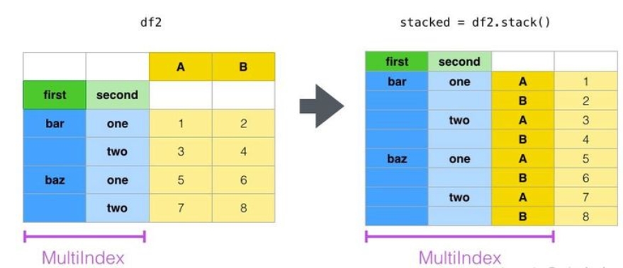
stacked = df2.stack()
stacked
first  second
bar    one     A   -1.922649
               B    1.871875
       two     A   -0.092881
               B    0.888805
baz    one     A   -0.663312
               B   -0.247438
       two     A    0.199572
               B    0.828977
dtype: float64
解压:
stacked.unstack()
|
|
A |
B |
| first |
second |
|
|
| bar |
one |
-1.922649 |
1.871875 |
| two |
-0.092881 |
0.888805 |
| baz |
one |
-0.663312 |
-0.247438 |
| two |
0.199572 |
0.828977 |
stacked.unstack(1)
|
second |
one |
two |
| first |
|
|
|
| bar |
A |
-1.922649 |
-0.092881 |
| B |
1.871875 |
0.888805 |
| baz |
A |
-0.663312 |
0.199572 |
| B |
-0.247438 |
0.828977 |
stacked.unstack(0)
|
first |
bar |
baz |
| second |
|
|
|
| one |
A |
-1.922649 |
-0.663312 |
| B |
1.871875 |
-0.247438 |
| two |
A |
-0.092881 |
0.199572 |
| B |
0.888805 |
0.828977 |
数据透视表
df = pd.DataFrame({'A': ['one', 'one', 'two', 'three'] * 3,
                   'B': ['A', 'B', 'C'] * 4,
                   'C': ['foo', 'foo', 'foo', 'bar', 'bar', 'bar'] * 2,
                   'D': np.random.randn(12),
                   'E': np.random.randn(12)})
df
|
A |
B |
C |
D |
E |
| 0 |
one |
A |
foo |
-1.123799 |
-1.098840 |
| 1 |
one |
B |
foo |
-1.913548 |
-0.119521 |
| 2 |
two |
C |
foo |
-0.639072 |
0.099824 |
| 3 |
three |
A |
bar |
-0.359609 |
1.435979 |
| 4 |
one |
B |
bar |
0.423144 |
0.761188 |
| 5 |
one |
C |
bar |
0.043997 |
0.928556 |
| 6 |
two |
A |
foo |
0.025243 |
-0.610217 |
| 7 |
three |
B |
foo |
-0.455484 |
-0.454505 |
| 8 |
one |
C |
foo |
2.812657 |
-0.321527 |
| 9 |
one |
A |
bar |
0.842464 |
-0.108601 |
| 10 |
two |
B |
bar |
0.075289 |
0.824193 |
| 11 |
three |
C |
bar |
0.352810 |
1.169305 |
pd.pivot_table(df, values='D', index=['A', 'B'], columns=['C'])
|
C |
bar |
foo |
| A |
B |
|
|
| one |
A |
0.842464 |
-1.123799 |
| B |
0.423144 |
-1.913548 |
| C |
0.043997 |
2.812657 |
| three |
A |
-0.359609 |
NaN |
| B |
NaN |
-0.455484 |
| C |
0.352810 |
NaN |
| two |
A |
NaN |
0.025243 |
| B |
0.075289 |
NaN |
| C |
NaN |
-0.639072 |